FishTaco Visualization
Visualization of functional shifts decomposition results obtained from applying FishTaco to you data can be done via a web-based application or by using a dedicated R package.
FishTacoPlot online plotting
For producing simple FishTaco plots from the functional shifts decomposition results generated by applying the FishTaco algorithm (via the python package), visit the online FishTacoPlot web-tool.
FishTacoPlot R package
Plotting the results obtained from applying FishTaco to you data can also be done by using the FishTacoPlot R package.
We used R for the plotting in order to take full advantage of the capabilities of the ggplot2 package.
We recommend downloading and installing R Studio before plotting, but it is not required.
The following packages need to be pre-installed in your R environment before using the FishTacoPlot package:
package-scales {scales}
ggplot2 {ggplot2}
grid {graphics}
In order to use the FishTacoPlot package:
Download the FishTacoPlot package from GitHub.
Install the package in your R terminal with the command:
install.packages(<path_to_package>, repos = NULL, type="source")Load the packages to your workspace with the command:
require(FishTacoPlot); require(ggplot2); require(scales); require(grid)Plot your results by using the function MultiFunctionTaxaContributionPlots.
Examples of using the FishTacoPlot package
In the <path_to_package>/examples directory, you can find results obtained by applying FishTaco to a healthy cohort of different body sites (HMP), and a type 2 diabetes cohort (T2D).
Metagenomic Comparative Analysis of Different Body Sites
An example of a FishTaco plot showing the species-level contributions to the functional enrichment of 3 pathways in tongue samples compared to cheek samples:
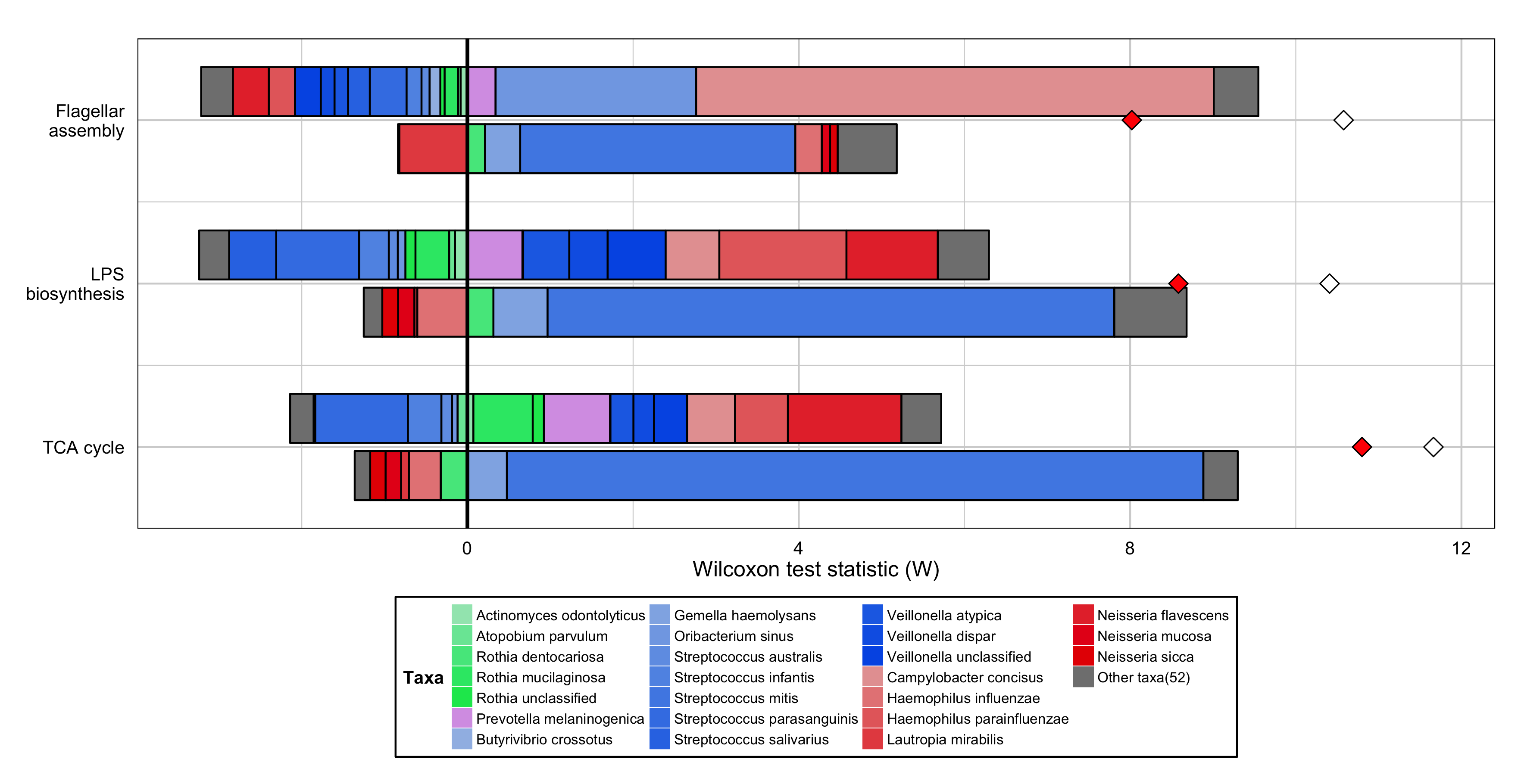
Generate this example by using the following commands:
p <- MultiFunctionTaxaContributionPlots(input_dir="<path_to_package>/examples", input_prefix="HMP_fishtaco",
input_taxa_taxonomy="<path_to_package>/examples/HMP_TAXONOMY.tab", sort_by="list", plot_type="bars",
input_function_filter_list=c("ko00020", "ko00540","ko02040"), add_predicted_da_markers=TRUE, add_original_da_markers=TRUE)

p <- p + scale_x_continuous(breaks=c(1, 2, 3), labels=c("TCA cycle", "LPS\nbiosynthesis", "Flagellar\nassembly")) +
guides(fill=guide_legend(nrow=7)) + ylab("Wilcoxon test statistic (W)") +
theme(plot.title=element_blank(), axis.title.x=element_text(size=12,colour="black",face="plain"),
axis.text.x=element_text(size=10,colour="black",face="plain"), axis.title.y=element_blank(),
axis.text.y=element_text(size=10,colour="black",face="plain"), axis.ticks.y=element_blank(),
axis.ticks.x=element_blank(), panel.grid.major.x = element_line(colour="light gray"), panel.grid.major.y = element_line(colour="light gray"),
panel.grid.minor.x = element_line(colour="light gray"), panel.grid.minor.y = element_line(colour="light gray"),
panel.background = element_rect(fill="transparent",colour=NA), panel.border = element_rect(fill="transparent",colour="black"),
legend.background=element_rect(colour="black"), legend.title=element_text(size=10), legend.text=element_text(size=8,face="plain"),
legend.key.size=unit(0.8,"line"), legend.margin=unit(0.1,"line"), legend.position="bottom")

ggsave <- ggplot2::ggsave; body(ggsave) <- body(ggplot2::ggsave)[-2]

ggsave("FishTaco_HMP.png", p, width=11.8, height=6.07, units="in")
Metagenomic Comparative Analysis of a Disease Cohort
An example of a FishTaco plot showing the genus-level contributions to the functional enrichment of 3 modules in type 2 diabetes patients compared to healthy controls:
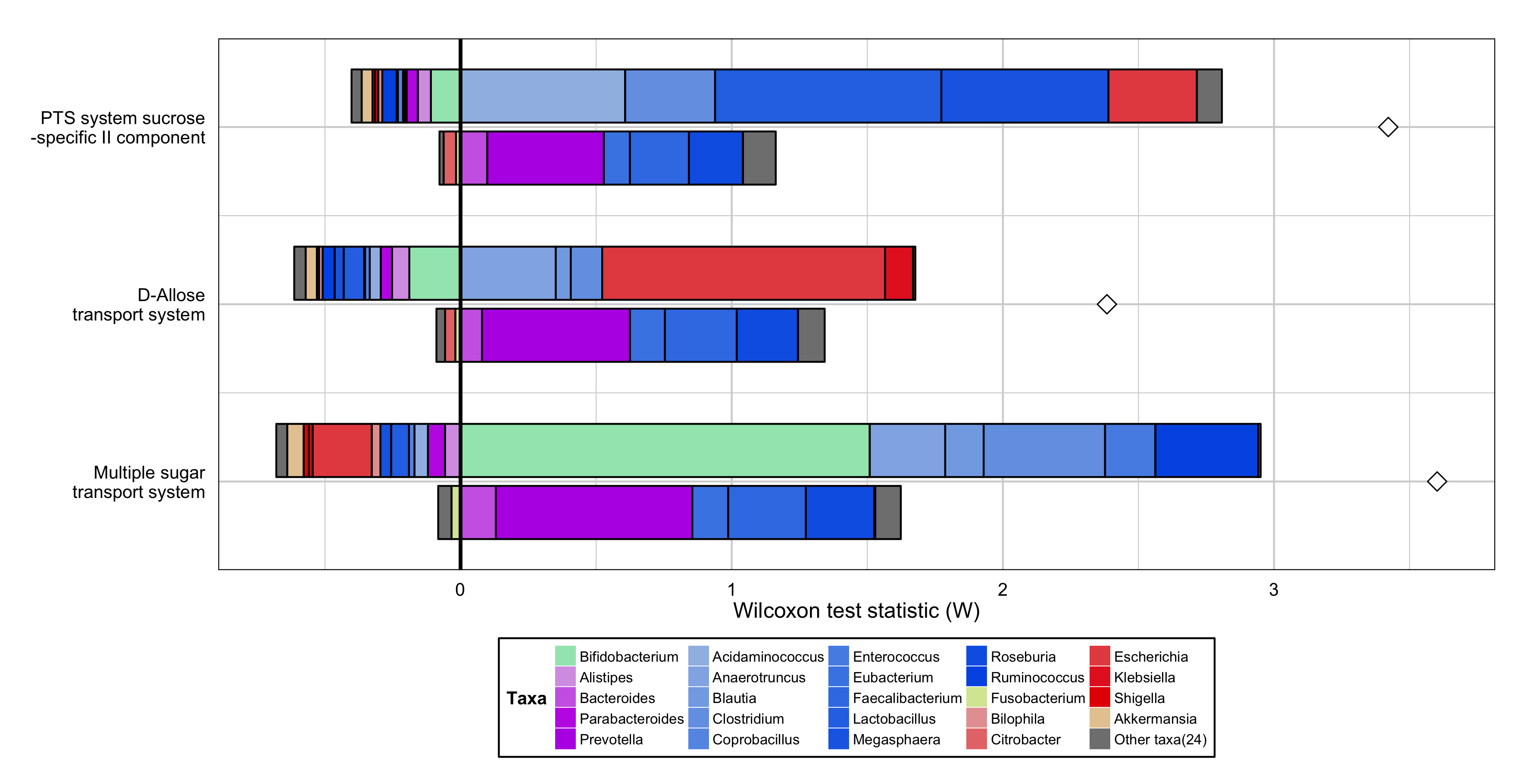
Generate this example by using the following commands:
p <- MultiFunctionTaxaContributionPlots(input_dir="<path_to_package>/examples", input_prefix="T2D_fishtaco",
input_taxa_taxonomy="<path_to_package>/examples/T2D_TAXONOMY.tab", sort_by="list", plot_type="bars",
input_function_filter_list=c("M00216", "M00217","M00269"), add_predicted_da_markers=TRUE)

p <- p + scale_x_continuous(breaks=c(1, 2, 3), labels=c("Multiple sugar\ntransport system", "D-Allose\ntransport system","PTS system sucrose\n -specific II component")) +
guides(fill = guide_legend(ncol=5)) + ylab("Wilcoxon test statistic (W)") +
theme(plot.title=element_blank(), axis.title.x=element_text(size=12,colour="black",face="plain"),
axis.text.x=element_text(size=10,colour="black",face="plain"), axis.title.y=element_blank(),
axis.text.y=element_text(size=10,colour="black",face="plain"), axis.ticks.y=element_blank(),
axis.ticks.x=element_blank(), panel.grid.major.x = element_line(colour="light gray"), panel.grid.major.y = element_line(colour="light gray"),
panel.grid.minor.x = element_line(colour="light gray"), panel.grid.minor.y = element_line(colour="light gray"),
panel.background = element_rect(fill="transparent",colour=NA), panel.border = element_rect(fill="transparent",colour="black"),
legend.background=element_rect(colour="black"), legend.title=element_text(size=10), legend.text=element_text(size=8,face="plain"),
legend.key.size=unit(0.8,"line"), legend.margin=unit(0.1,"line"), legend.position="bottom")

ggsave <- ggplot2::ggsave; body(ggsave) <- body(ggplot2::ggsave)[-2]

ggsave("FishTaco_T2D.png", p, width=11.8, height=6.07, units="in")